Data source importance • sealIPM

library(sealIPM)
library(tidyverse)
#> ── Attaching core tidyverse packages ──────────────────────── tidyverse 2.0.0 ──
#> ✔ dplyr     1.2.1     ✔ readr     2.2.0
#> ✔ forcats   1.0.1     ✔ stringr   1.6.0
#> ✔ ggplot2   4.0.3     ✔ tibble    3.3.1
#> ✔ lubridate 1.9.5     ✔ tidyr     1.3.2
#> ✔ purrr     1.2.2     
#> ── Conflicts ────────────────────────────────────────── tidyverse_conflicts() ──
#> ✖ dplyr::filter() masks stats::filter()
#> ✖ dplyr::lag()    masks stats::lag()
#> ℹ Use the conflicted package (<http://conflicted.r-lib.org/>) to force all conflicts to become errors
library(tinytable)
library(priorsense)
library(posterior)
#> This is posterior version 1.7.0
#> 
#> Attaching package: 'posterior'
#> 
#> The following objects are masked from 'package:stats':
#> 
#>     mad, sd, var
#> 
#> The following objects are masked from 'package:base':
#> 
#>     %in%, match
library(ggdist)
library(patchwork)

The data described in Vanko et al. 2026 is available in the package as grey_seal_data

data(grey_seal_data)

The model has the following data sources:

aerial counts: aerial
total hunting counts in Sweden: harvest_bags_finland
total hunting counts in Finland: harvest_bags_finland
age/sex composition of hunted samples in Sweden: hunting_comp_sweden
age/sex composition of hunted samples in Finland: hunting_comp_finland
bycatch composition (combined): bycatch
pregnancy observations: pregnancy
reproductive signs: reproductive_signs

We first fit the model with all the data sources.

fit_full <- fit_ipm(
    data = grey_seal_data,
    species = "grey",
    years = 2005:2010,
    iter_warmup = 1000,
    iter_sampling = 500,
    chains = 10,
    seed = 123,
    refresh = 0
)

Next we check the likelihood sensitivity for each source separately. We focus on the posterior of the population in the final year: population_total_final

sources <- c(
    "aerial",
    "harvest_bags_finland",
    "harvest_bags_sweden",
    "hunting_comp_finland",
    "hunting_comp_sweden",
    "bycatch",
    "pregnancy",
    "reproductive_signs"
)

source_likelihood_sens <- map(
    sources,
    ~ powerscale_sensitivity(
        fit_full$fit,
        component = "likelihood",
        variable = "population_total_final",
        likelihood_selection = .x
    ) |>
        mutate(source = .x)
) |>
    list_rbind() |>
    select(source, likelihood, -prior, -diagnosis, -variable) |>
    arrange(likelihood) |>
rename(Source = source, "Likelihood sensitivity" = likelihood)

source_likelihood_sens |> tt(digits = 1)

Source	Likelihood sensitivity
pregnancy	0.003
harvest_bags_finland	0.007
harvest_bags_sweden	0.008
reproductive_signs	0.015
bycatch	0.017
hunting_comp_finland	0.021
hunting_comp_sweden	0.048
aerial	0.189

Pregnancy signs exhibits much lower likelihood sensitivity than others. Based on this, we fit a reduced model excluding that source.

data_no_pregnancy <- grey_seal_data
data_no_pregnancy[["pregnancy_status"]] <- tibble(
    Year = numeric(0),
    Status = numeric(0)
)


fit_no_pregnancy <- fit_ipm(
    data = data_no_pregnancy,
    species = "grey",
    years = 2005:2010,
    iter_warmup = 1000,
    iter_sampling = 500,
    chains = 10,
    seed = 123,
    refresh = 0
)

Next we compare the full and reduced models on their forecasts:

We first specify data to use for forecasting.

future_data <- tibble(
    Herring_GoF_BP = c(0, 0),
    Herring_GoB = c(0, 0),
    Sweden_Quota = c(1000, 1000),
    Finland_Quota = c(1000, 1000)
)

We then run the forecast for each of the models.

forecast_full <- forecast_ipm(
    fit_full,
    future_data = future_data,
    species = "grey"
)
#> Running standalone generated quantities after 10 MCMC chains, all chains in parallel ...
#> 
#> Chain 1 finished in 0.2 seconds.
#> Chain 2 finished in 0.2 seconds.
#> Chain 3 finished in 0.2 seconds.
#> Chain 4 finished in 0.2 seconds.
#> Chain 5 finished in 0.2 seconds.
#> Chain 6 finished in 0.2 seconds.
#> Chain 9 finished in 0.1 seconds.
#> Chain 7 finished in 0.2 seconds.
#> Chain 8 finished in 0.2 seconds.
#> Chain 10 finished in 0.2 seconds.
#> 
#> All 10 chains finished successfully.
#> Mean chain execution time: 0.2 seconds.
#> Total execution time: 0.5 seconds.

no_pregnancy_forecast <- forecast_ipm(
    fit_no_pregnancy,
    future_data = future_data,
    species = "grey"
)
#> Running standalone generated quantities after 10 MCMC chains, all chains in parallel ...
#> 
#> Chain 1 finished in 0.2 seconds.
#> Chain 2 finished in 0.2 seconds.
#> Chain 3 finished in 0.2 seconds.
#> Chain 4 finished in 0.3 seconds.
#> Chain 5 finished in 0.2 seconds.
#> Chain 6 finished in 0.2 seconds.
#> Chain 7 finished in 0.2 seconds.
#> Chain 8 finished in 0.2 seconds.
#> Chain 9 finished in 0.2 seconds.
#> Chain 10 finished in 0.2 seconds.
#> 
#> All 10 chains finished successfully.
#> Mean chain execution time: 0.2 seconds.
#> Total execution time: 0.6 seconds.

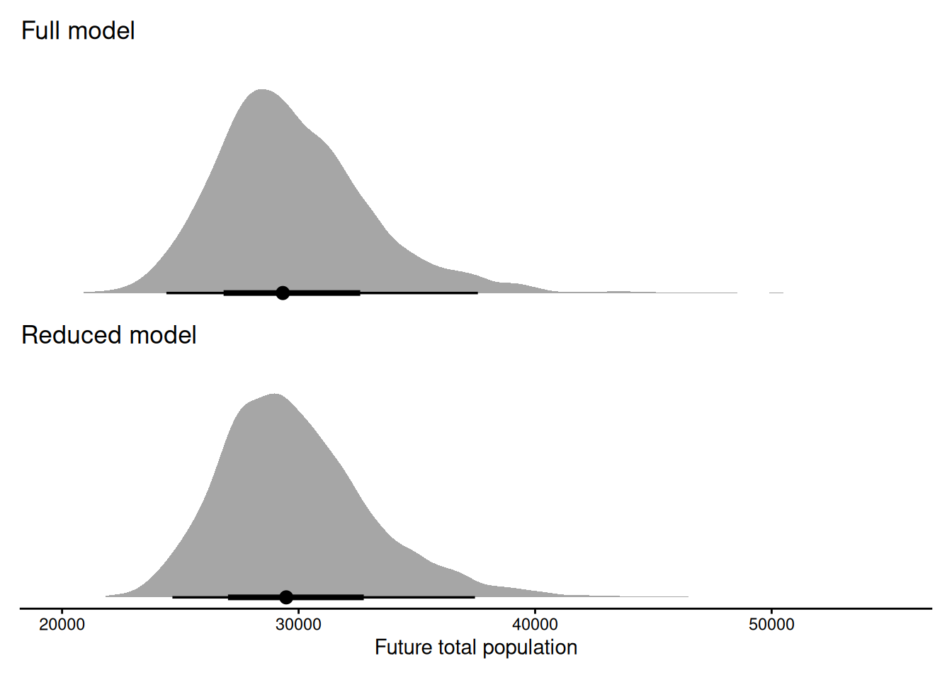
And see how the models forecast the future population. Here we can judge whether the difference between the full and reduced models is meaningful, or if we consider dropping the source.

plot_full <- forecast_full$draws("population_total_future", format = "draws_df") |>
    ggplot(aes(x = `population_total_future[2]`)) +
    stat_halfeye() +
    xlim(20000, 55000) +
    ggtitle("Full model")

plot_reduced <- no_pregnancy_forecast$draws("population_total_future", format = "draws_df") |>
    ggplot(aes(x = `population_total_future[2]`)) +
    stat_halfeye() +
    xlim(20000, 55000) +
    ggtitle("Reduced model")

plot_full / plot_reduced +
    plot_layout(axes = "collect") &
    theme_classic() &
    theme(
        axis.text.y = element_blank(),
        axis.title.y = element_blank(),
        axis.line.y = element_blank(),
        axis.ticks.y = element_blank()) &
    xlab("Future total population")
#> Warning: Removed 1 row containing missing values or values outside the scale range
#> (`stat_slabinterval()`).