Exercises

Part 1: Posterior draws objects

For this set of exercises we will use draws from the classic eight schools model. These draws are included in both posterior and ArviZ.

Understanding draws objects

Inspect the posterior object. How many chains, iterations and variables does it contain?

eight_schools_draws.sizes["chain"]

eight_schools_draws.sizes["draw"]

len(eight_schools_draws.data_vars)

Subsetting draws

Extract only the first chain.

eight_schools_draws.sel(chain=0)

Extract only the first 10 iterations, from all the chains.

eight_schools_draws.sel(draw=slice(0, 10))

Thinning draws

Thin the draws so that only half of the draws are included. Then try automatic thinning.

az.thin(eight_schools_draws, factor=2)

az.thin(eight_schools_draws)

Summarising draws

Extract the variable mu and summarise it via mean and sd.

# XXX do we want to show this?
az.summary(eight_schools_draws, var_names=["mu"], kind="stats")

   mean   sd eti89_lb eti89_ub
mu  4.3  3.3    -0.75      9.4

## or this?
az.summary(eight_schools_draws, var_names=["mu"], kind="stats")[["mean", "sd"]]

   mean   sd
mu  4.3  3.3

Creating new variables

Create a new variable that is the difference between school 1 and school 2 means. Call it diff_1_2. Do the same with school 3 and school 4. Then summarise these new variables with median, 0.3 and 0.7 quantiles.

The simplest version is to call az.summary() with the kind argument set to "stats_median" and the ci_prob argument set to 0.40.

import xarray as xr

diff_1_2 = eight_schools_draws["theta"].isel(school=1) - eight_schools_draws["theta"].isel(school=0)
diff_3_4 = eight_schools_draws["theta"].isel(school=3) - eight_schools_draws["theta"].isel(school=2)

diffs = xr.Dataset({"diff_1_2": diff_1_2, "diff_3_4": diff_3_4})

az.summary(diffs, kind="stats_median", ci_prob=0.40)

         median mad eti40_lb eti40_ub
diff_1_2  -0.33   2     -2.3     0.69
diff_3_4   0.15   2    -0.96      1.9

But a more explicit version is to do.

import pandas as pd
result = pd.DataFrame({
    "median": diffs.median(dim=["chain", "draw"]).to_pandas(),
    "q30": diffs.quantile(0.3, dim=["chain", "draw"]).to_pandas(),
    "q70": diffs.quantile(0.7, dim=["chain", "draw"]).to_pandas(),
})

result

            median       q30       q70
diff_1_2 -0.331771 -2.276892  0.686635
diff_3_4  0.154759 -0.962139  1.931608

Optionally you can use .sel and reference the school by name like eight_schools_draws["theta"].sel(school="Choate")

Marginal posteriors

Plot the marginal posteriors for the school means.

az.plot_forest(eight_schools_draws, var_names=["theta"])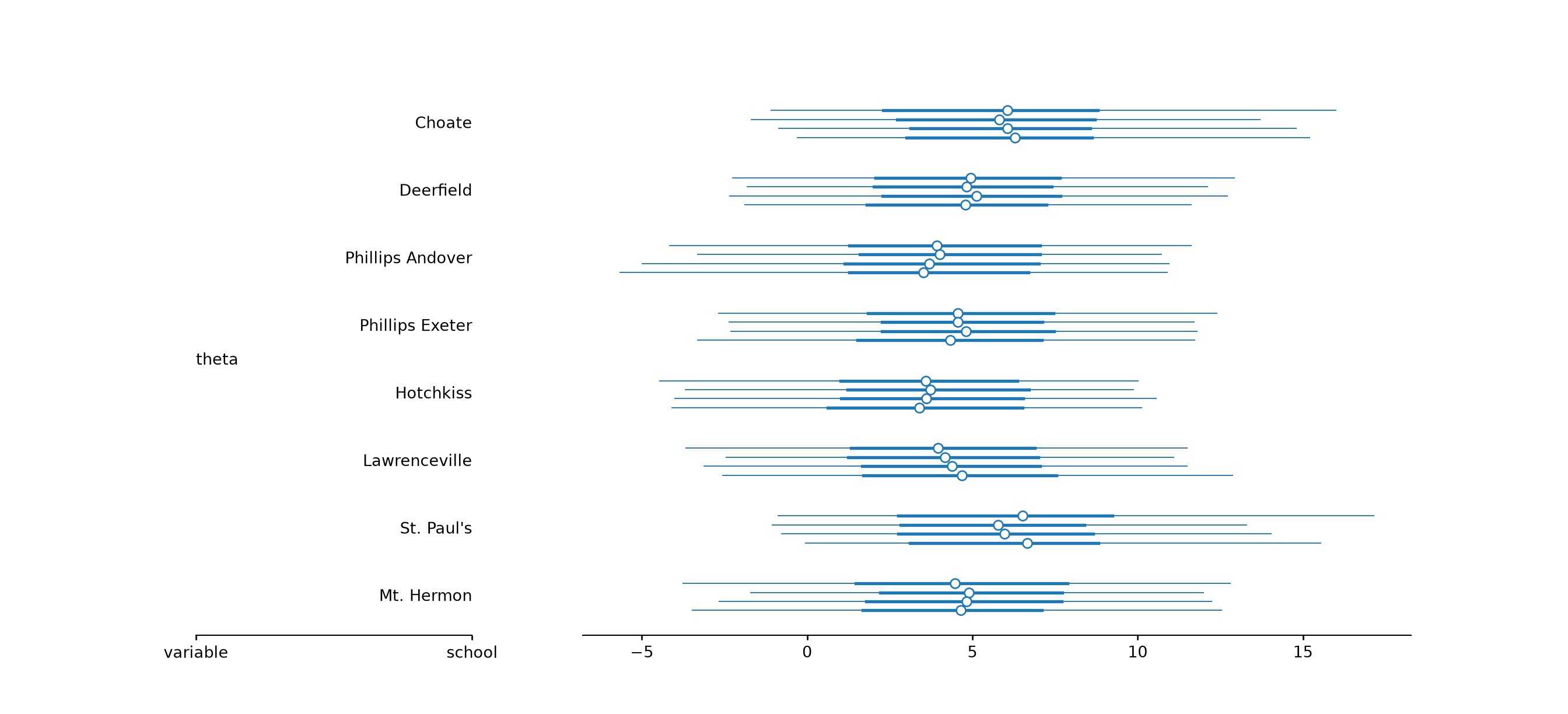

Pairs plot

Plot the variables mu and tau in an pairs plot.

az.plot_pair(eight_schools_draws, var_names=["mu", "tau"])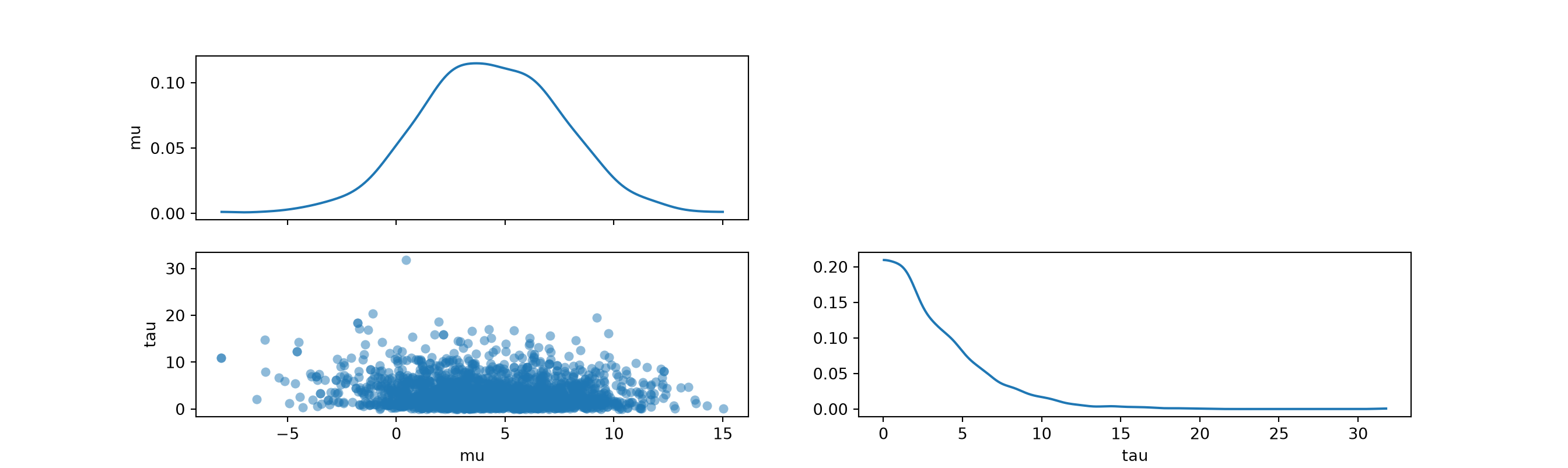

Part 2: Convergence diagnostics and uncertainty

R-hat

Calculate the R-hat for all the variables in the model. Which variables have high R-hat (> 1.01)?

az.rhat(eight_schools_draws)

Effective sample size (ESS)

Calculate the bulk and tail ESS for all the variables in the model.

az.summary(eight_schools_draws)[["ess_bulk", "ess_tail"]]

                           ess_bulk  ess_tail
mu                             2114      1219
theta_t[Choate]                2249      1467
theta_t[Deerfield]             2638      1512
theta_t[Phillips Andover]      2689      1511
theta_t[Phillips Exeter]       2431      1586
theta_t[Hotchkiss]             2190      1545
theta_t[Lawrenceville]         2372      1297
theta_t[St. Paul's]            1980      1391
theta_t[Mt. Hermon]            2420      1538
tau                             833       712
theta[Choate]                  2195      1443
theta[Deerfield]               2321      1499
theta[Phillips Andover]        2108      1504
theta[Phillips Exeter]         2288      1434
theta[Hotchkiss]               2103      1609
theta[Lawrenceville]           2364      1662
theta[St. Paul's]              1431      1629
theta[Mt. Hermon]              2187      1569

Monte Carlo standard error

Calculate the mean of each variable, and also the Monte Carlo standard error of the mean.

az.summary(eight_schools_draws)[["mean", "mcse_mean"]]

                            mean mcse_mean
mu                           4.3     0.072
theta_t[Choate]             0.33     0.021
theta_t[Deerfield]           0.1     0.018
theta_t[Phillips Andover]  -0.08     0.019
theta_t[Phillips Exeter]    0.05     0.019
theta_t[Hotchkiss]         -0.15      0.02
theta_t[Lawrenceville]     -0.03     0.019
theta_t[St. Paul's]         0.35     0.022
theta_t[Mt. Hermon]         0.05      0.02
tau                          3.5     0.091
theta[Choate]                6.1      0.12
theta[Deerfield]             4.9     0.097
theta[Phillips Andover]      3.8      0.12
theta[Phillips Exeter]       4.6       0.1
theta[Hotchkiss]             3.6       0.1
theta[Lawrenceville]         4.3       0.1
theta[St. Paul's]            6.2      0.14
theta[Mt. Hermon]            4.7      0.12

Then do the same for the 0.05 and 0.95 quantiles. Think about how the Monte Carlo standard error might influence how you report the quantiles.

mcse_q05 = az.mcse(eight_schools_draws, method="quantile", prob=0.05).ds.expand_dims(summary=["mcse_5%"])
mcse_q95 = az.mcse(eight_schools_draws, method="quantile", prob=0.95).ds.expand_dims(summary=["mcse_95%"])

eti_05 = (
    az.eti(eight_schools_draws, prob=0.90)
    .ds.rename({"ci_bound": "summary"})
    .assign_coords(summary=["eti90_lb", "eti90_ub"])
)

summary = xr.concat([mcse_q05, mcse_q95, eti_05], dim="summary")

az.dataset_to_dataframe(summary, sample_dims=["summary"]).T

                            mcse_5%  mcse_95%  eti90_lb   eti90_ub
mu                         0.244848  0.144510 -0.918682   9.530723
theta_t[Choate]            0.072708  0.041516 -1.443312   1.967369
theta_t[Deerfield]         0.042073  0.050981 -1.424052   1.701920
theta_t[Phillips Andover]  0.058658  0.052118 -1.656461   1.432035
theta_t[Phillips Exeter]   0.059665  0.062823 -1.486306   1.579305
theta_t[Hotchkiss]         0.047558  0.047945 -1.656586   1.353910
theta_t[Lawrenceville]     0.050866  0.035970 -1.656941   1.503961
theta_t[St. Paul's]        0.096855  0.051169 -1.285794   1.927415
theta_t[Mt. Hermon]        0.050794  0.048198 -1.606512   1.620798
tau                        0.036199  0.337611  0.206986   9.729145
theta[Choate]              0.280439  0.459703 -1.279904  15.268796
theta[Deerfield]           0.280272  0.410776 -2.256395  12.959238
theta[Phillips Andover]    0.445232  0.166002 -4.865964  11.342719
theta[Phillips Exeter]     0.380658  0.300268 -2.976054  12.214636
theta[Hotchkiss]           0.383721  0.255297 -4.519310  10.358722
theta[Lawrenceville]       0.362746  0.228841 -3.208492  11.797317
theta[St. Paul's]          0.223813  0.494425 -0.814740  15.327724
theta[Mt. Hermon]          0.433716  0.314653 -3.376179  12.817132

Pareto diagnostics

Calculate the minimum sample size for stable estimates for each variable in the model. Which has the highest minimum sample size?

eight_schools_draws.azstats.pareto_min_ss()

Part 3: Model evaluation and critique

We can generate prior predictions from the eight schools model, using the following function.

Generate 1000 prior predictive draws, and plot the distributions for each school. Try with different mu_prior_sd and tau_prior_sd values (e.g. 1, 10, 100).

az.plot_forest(eight_schools_prior(ndraws=1000, mu_prior_sd=1, tau_prior_sd=1), group="prior", var_names=["yrep"])

az.plot_forest(eight_schools_prior(ndraws=1000, mu_prior_sd=0.01, tau_prior_sd=1), group="prior", var_names=["yrep"])

az.plot_forest(eight_schools_prior(ndraws=1000, mu_prior_sd=100, tau_prior_sd=1), group="prior", var_names=["yrep"])

az.plot_forest(eight_schools_prior(ndraws=1000, mu_prior_sd=1, tau_prior_sd=0.01), group="prior", var_names=["yrep"])

az.plot_forest(eight_schools_prior(ndraws=1000, mu_prior_sd=1, tau_prior_sd=100), group="prior", var_names=["yrep"])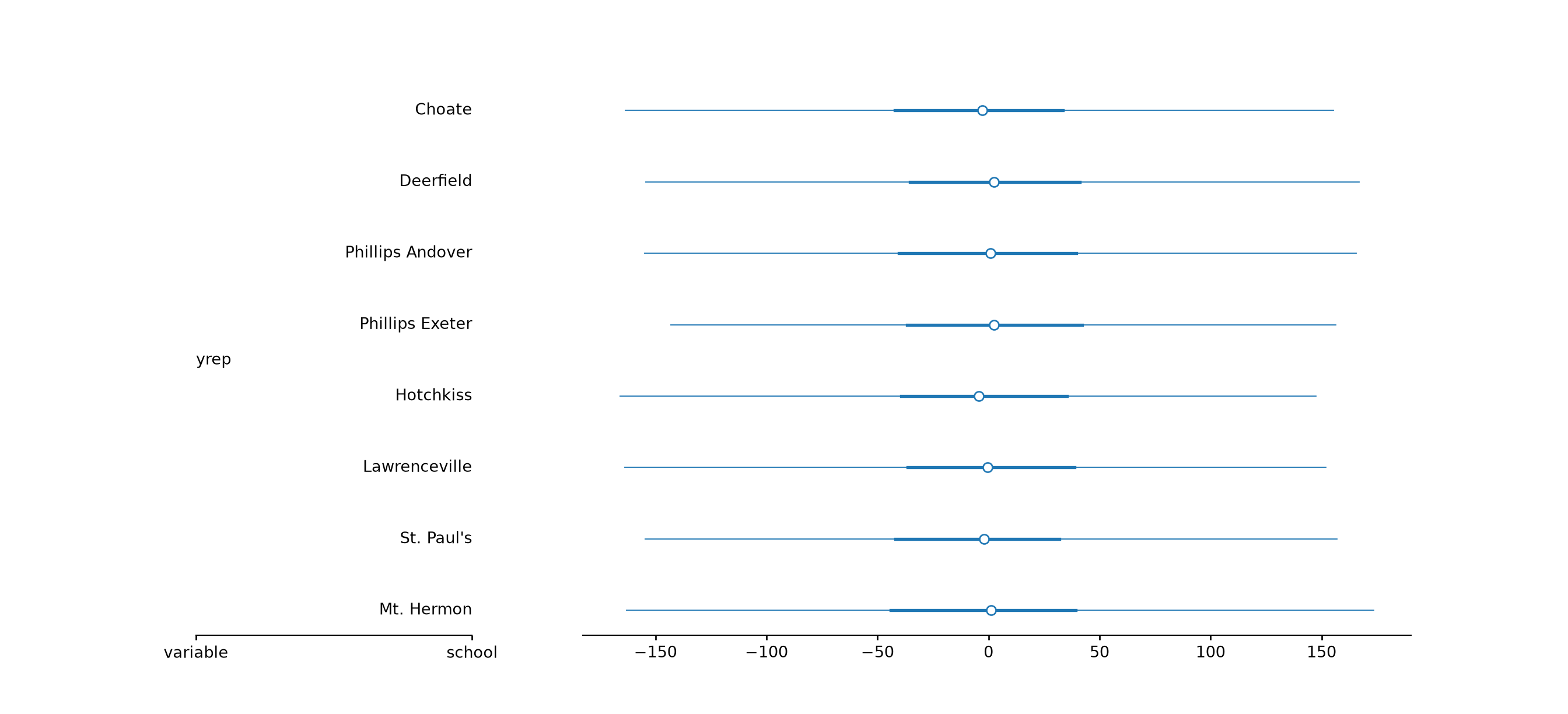

Posterior predictive checks

We can create posterior predictive draws from our posterior draws and plot against our actual observations.

Plot the posterior predictions on top of the actual observations. Then use the PIT-ECDF plot.

y = np.array([28,  8, -3,  7, -1,  1, 18, 12])
posterior_predictive_draws["observed_data"]["yrep"] = xr.DataArray(y, dims=["school"])
az.plot_ppc_pit(posterior_predictive_draws, var_names=["yrep"])

Sensitivity checks

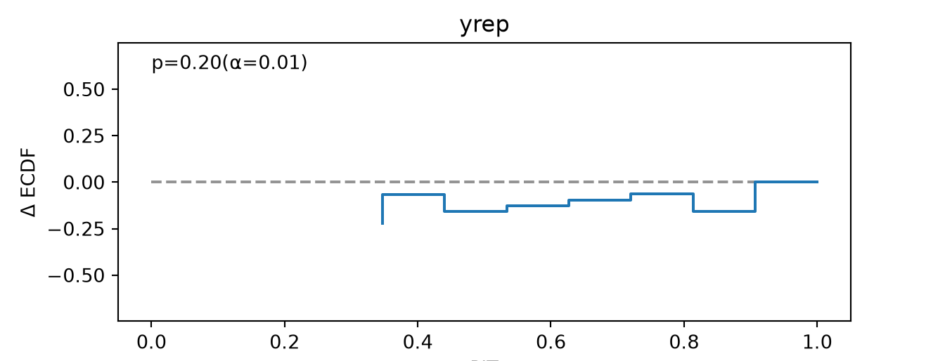
Check for prior and likelihood sensitivity in the eight schools model. First check by power-scaling all priors jointly, then select only the “mu” and only the “tau” prior separately.

az.psense_summary(dt)

We detected potential issues. For more information on how to interpret the results, please check
https://arviz-devs.github.io/EABM/Chapters/Sensitivity_checks.html#interpreting-sensitivity-diagnostics-summary
or read original paper https://doi.org/10.1007/s11222-023-10366-5
                            prior  likelihood                                 diagnosis
mu                          2.230       0.093             potential prior-data conflict
theta_t[Choate]             0.833       0.040  potential strong prior / weak likelihood
theta_t[Deerfield]          0.384       0.010  potential strong prior / weak likelihood
theta_t[Phillips Andover]   0.503       0.021  potential strong prior / weak likelihood
theta_t[Phillips Exeter]    0.388       0.013  potential strong prior / weak likelihood
theta_t[Hotchkiss]          0.739       0.034  potential strong prior / weak likelihood
theta_t[Lawrenceville]      0.368       0.016  potential strong prior / weak likelihood
theta_t[St. Paul's]         0.854       0.042  potential strong prior / weak likelihood
theta_t[Mt. Hermon]         0.264       0.009  potential strong prior / weak likelihood
tau                        12.067       0.051             potential prior-data conflict
theta[Choate]               3.189       0.084             potential prior-data conflict
theta[Deerfield]            3.105       0.064             potential prior-data conflict
theta[Phillips Andover]     2.685       0.039  potential strong prior / weak likelihood
theta[Phillips Exeter]      1.938       0.079             potential prior-data conflict
theta[Hotchkiss]            2.044       0.041  potential strong prior / weak likelihood
theta[Lawrenceville]        2.152       0.048  potential strong prior / weak likelihood
theta[St. Paul's]           4.373       0.075             potential prior-data conflict
theta[Mt. Hermon]           3.162       0.053             potential prior-data conflict

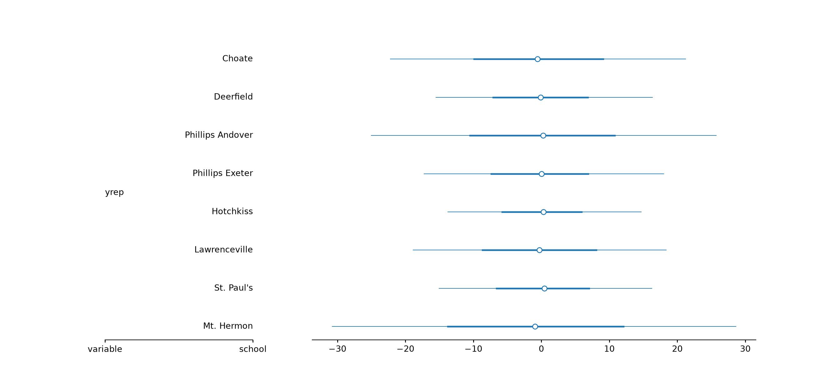
Next plot sensitivity using as density plots. Plot only the mu and tau variables.

az.plot_psense_dist(dt, var_names=["mu", "tau"])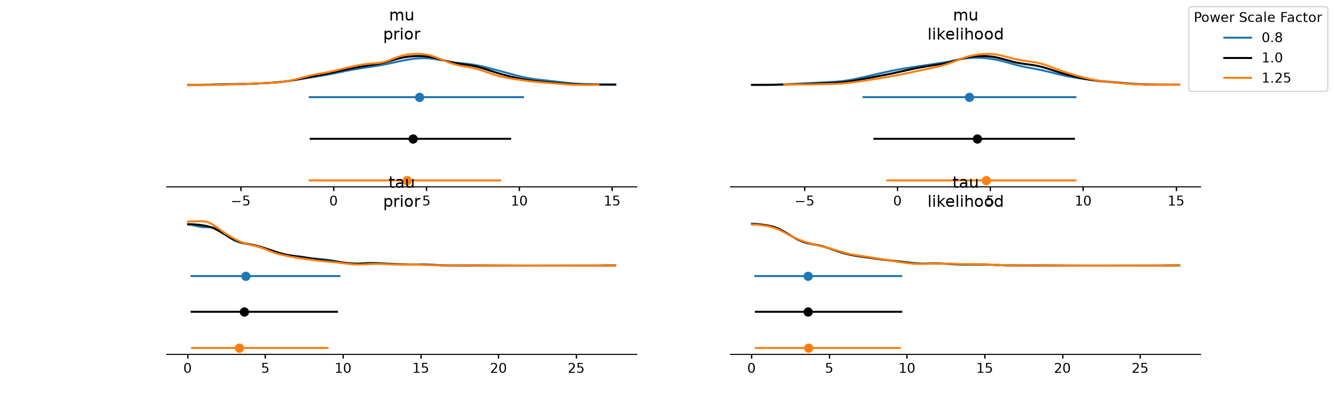

Part 4: Bringing it all together

We have provided four sets of posterior draws from hierarchical models of observed migratory bird counts recorded between 2000 and 2020 at the Hanko Bird Observatory (Halias).

For species \(j\),

\(y \sim \mathrm{Poisson}(\lambda_j)\)

\(y \sim \mathrm{NegativeBinomial}(\lambda_j, \phi).\)

The species-specific abundances are linked through a hierarchical prior,

\(\log(\lambda_j) \sim \mathrm{Normal}(\mu, \sigma)\)

where \(\mu\) represents the average abundance across species and \(\sigma\) controls the amount of pooling between species.

Your task is to explore the posterior draws and diagnostic outputs for the four fitted models.

As you work through the diagnostics, try to identify which model corresponds to each of the following situations:

Convergence issues caused by poor chain mixing (for example, insufficient warmup).
Inadequate fit to the data caused by the choice of observation model, shown by posterior predictive checks.
Issues caused by priors in conflict with the likelihood.
No major issues, although there is still room for model improvement.

Use posterior summaries, convergence diagnostics, posterior predictive checks, and sensitivity analyses to guide your investigation.

You can also look at the Stan model (birds_per_year.stan) and consider how you might improve it.